
Fil:Equipotential by Zureks.png

Størrelse på denne forhåndsvisningen: 366 × 600 piksler. Andre oppløsninger: 146 × 240 piksler | 639 × 1 047 piksler.
Opprinnelig fil (639 × 1 047 piksler, filstørrelse: 111 KB, MIME-type: image/png)
| Denne filen er fra Wikimedia Commons og kan brukes av andre prosjekter. Informasjonen fra filbeskrivelsessiden vises nedenfor. |
Beskrivelse
| Beskrivelse |
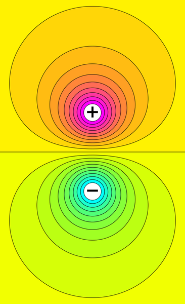
English: Voltage distribution between two electrically charged spheres (purple = positive voltage, blue = negative voltage). The black curves show equipotential contours. |
|||
| Dato | ||||
| Kilde | Eget verk | |||
| Opphavsperson | Zureks | |||
| Andre versjoner |
|


Source code
The image can be created with Python Matplotlib using the following code:
import numpy as np
from matplotlib import pyplot as plt
from matplotlib import colors

cmap = colors.ListedColormap([np.clip((2*x, 2*(1-x), 4*(x-0.5)**2), 0, 1) for x in np.linspace(0., 1., 256)])

w, h = 639, 1047
xmax = 2.36
ymax = xmax * float(h) / float(w)
vmax = 0.78
y0 = 1.0
nlevels = 21
levels = np.linspace(-vmax, vmax, nlevels)
X, Y = np.mgrid[-xmax:xmax:250j, -ymax:ymax:800j]

# potential of two point charges
V  = 1.0 / np.maximum(np.sqrt(X**2 + (Y - y0)**2), 1e-2)
V -= 1.0 / np.maximum(np.sqrt(X**2 + (Y + y0)**2), 1e-2)

# rescale potential globally to make contour areas similar
V = (np.sqrt(1 + V * V) - 1) / V

plt.figure(figsize=(w/90., h/90.)).add_axes([0, 0, 1, 1])
contf = plt.contourf(X, Y, V, levels=levels, cmap=cmap,
         vmin=-vmax*(nlevels-1.)/nlevels, vmax=vmax*(nlevels-1.)/nlevels)
cont = plt.contour(X, Y, V, levels=contf.levels, colors='k', linestyles='solid')

plt.xticks([]), plt.yticks([])
plt.gca().set_aspect(aspect='equal')
plt.gca().axis('off')
plt.text(0, -y0, u'\u2212', size=48,fontweight='bold', ha='center', va='center')
plt.text(0, y0, '+', size=48,fontweight='bold', ha='center', va='center')
plt.savefig('Equipotential_of_dipole.png')
Lisensiering
| Denne filen er gjort tilgjengelig under lisensen Creative Commons CC0 1.0 Universal Fristatus-erklæring. | |
| Personen som koblet et verk med dette dokumentet har tilegnet arbeidet til allmennheten ved, i den utstrekning loven tillater det, å avstå fra alle de rettigheter vedkommende skulle hatt ifølge opphavsrettsloven og andre relaterte eller nærliggende juridiske rettigheter. Verk under CC0 krever ikke attributtering. Ved bruk av verket trenger du ikke å få godkjennelse fra opphavspersonen.
|
Filhistorikk
Klikk på et tidspunkt for å vise filen slik den var på det tidspunktet.
| Dato/klokkeslett | Miniatyrbilde | Dimensjoner | Bruker | Kommentar | |
|---|---|---|---|---|---|
| nåværende | 16. mai 2018 kl. 23:09 | | 639 × 1 047 (111 KB) | Geek3 | Replaced with analytically computed precise contour shapes. The old version which came from an FEM simulation had significant errors towards the edges, possibly because the simulation volume was chosen too small. The potential dropped much too slowly towards the image edges. In contrast, the analytic solution is very simple, as the potential is just the linear sum of two 1/r potentials. |
| 11. apr. 2010 kl. 18:37 |  | 639 × 1 047 (32 KB) | Zureks | {{Information |Description={{en|1=Voltage distribution between two electrically charged spheres (purple = positive voltage, blue = negative voltage). The black curves show equipotential contours.}} |Source={{own}} |Author=Zureks |Date=2010 |
Filbruk
Den følgende siden bruker denne filen:
Global filbruk
Følgende andre wikier bruker denne filen:
- Bruk i ar.wikipedia.org
- Bruk i be-tarask.wikipedia.org
- Bruk i cs.wikipedia.org
- Bruk i fi.wikipedia.org
- Bruk i fr.wikipedia.org
- Bruk i ht.wikipedia.org
- Bruk i kk.wikipedia.org
- Bruk i ko.wikipedia.org
- Bruk i oc.wikipedia.org
- Bruk i ru.wikipedia.org
- Bruk i sl.wikipedia.org
- Bruk i uk.wikipedia.org
- Bruk i www.wikidata.org
- Bruk i zh.wikipedia.org